Intro

In Part 1 of our vLLM for beginners Series, we covered the fundamentals—core concepts and terminology behind vLLM’s architecture. In Part 2, we go deeper into what makes vLLM excel at performance: features like PagedAttention, attention backends, prefill & decode management, and more.

💡This series is about building a strong foundation in vLLM—understanding how it works and why it’s becoming the de facto choice for LLM serving.

So here’s to more insights in the world of LLM inference🫶🏻

How Features Work in vLLM Architecture 🚀

When I first explored vLLM’s features, they felt all over the place. Everything sounded important, but it wasn’t easy to see how they fit together. This is why I decided to group them by both their functionality and architecture layer.
A way, for us, to make sense of it all, and keep structure in this write-up.

I. Memory Management Layer

On top of KV Cache Offloading from GPU to CPU or Intelligent Routing that redirects requests to maximize KV cache reuse. vLLM has other mechanisms to optimize the memory.

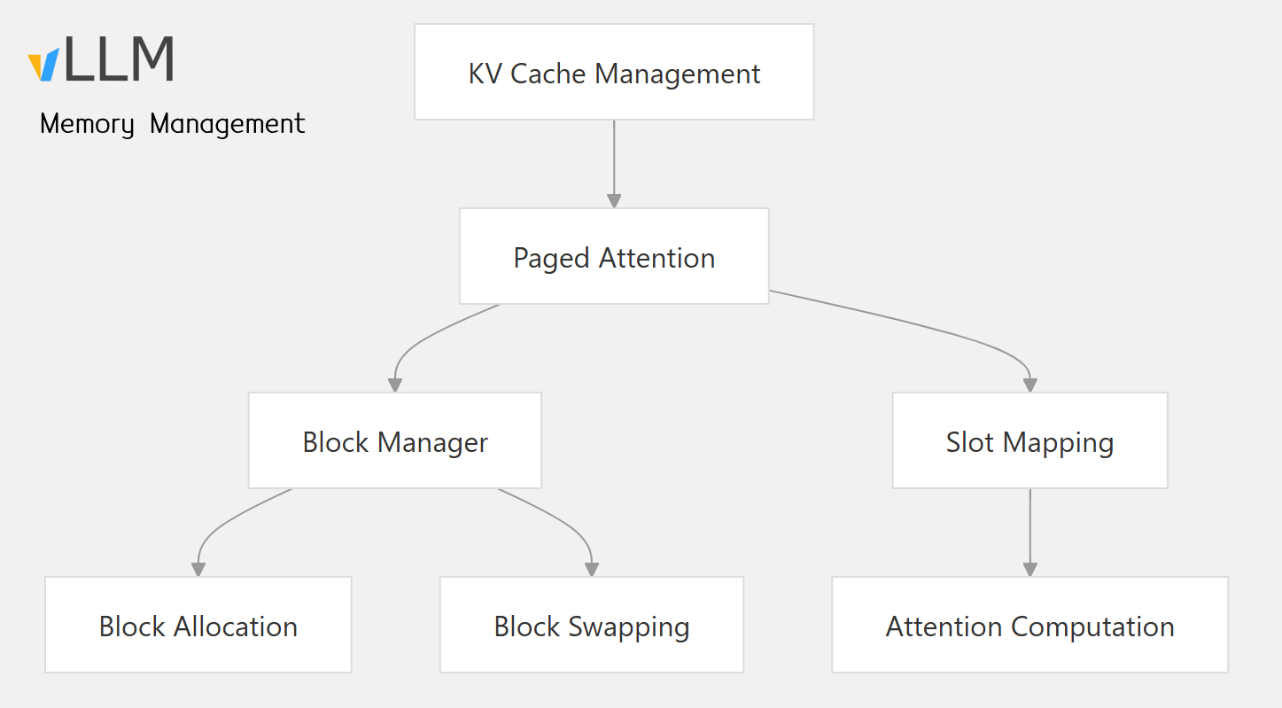
1. Paged Attention

PagedAttention is a core innovation in vLLM that which treats the KV cache like a virtual memory as described below

• Splits KV cache into (non-contiguous) fixed-size blocks instead of one large tensor.
• Uses a lookup table to fetch only needed blocks per attention step.
• Reduces memory fragmentation, imitating OS memory swapping, supports larger batches.
• Enables KV sharing between parallel similar prompts (many-to-one mapping between logical ➡️ physical blocks).
• PagedAttention has a shape of (2, num_blocks, block_size, num_kv_heads, head_size)

II. Scheduling and Batching Layer

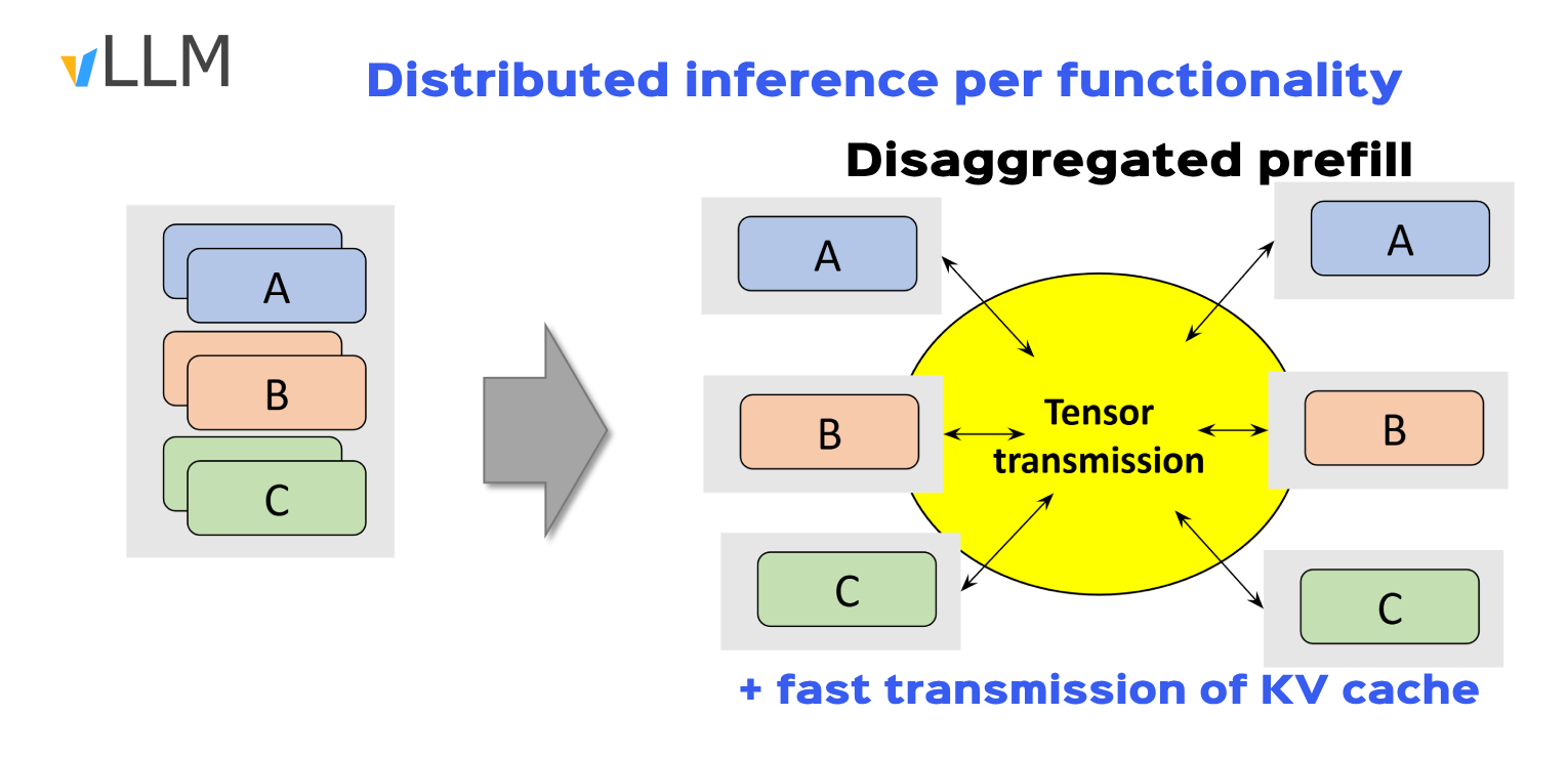
1. Disaggregated Prefill(NVIDIA)

Disaggregated Prefill improves time to first token by processing multiple partial prefills concurrently across GPU resources more efficiently. A sort of parallel distributed prefill across vLLM instances through NCCL GPU-GPU link.

Key Problems:

• Keeping prefill and decode in the same node leads to contention and high in-token latency.
• Having multi modal functionalities on a same node (vision models vs. LLM/ heterogeneous HW) creates contention.

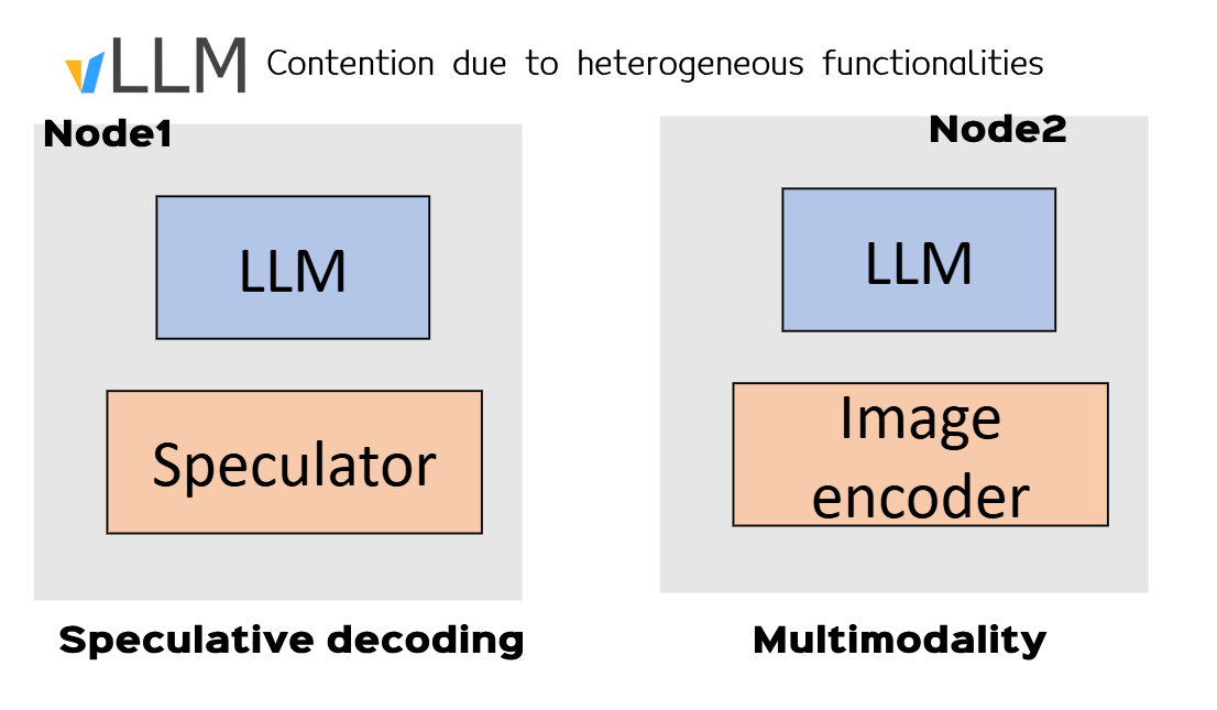
• Running one functionality per instance optimizes the time to first token and inter-token latency
• Ex: 1️⃣ vLLm node1 running prefill, node2 decode, node3 vision model and so on, while keeping kv_cache transfer
• Use case: speculative decoding and multimodality

2. Chunked Prefill

Chunked prefill is a technique for breaking a long input into smaller parts so the model can start generating responses sooner—without waiting for the entire input to process first. It improvements include:

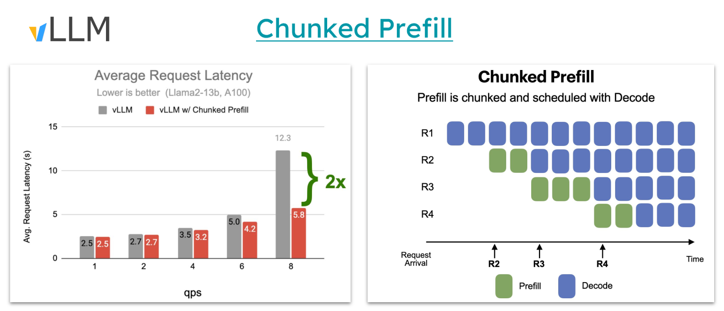
• Limit the number of batched tokens to maintain low latency and reduce TTFT (up to 30%)
• Enforce the batching of both prefill and decode requests together (up to x1.4 ITL)

3. Prefix Caching

Automatic Prefix Caching (APC) improves performance when processing multiple prompts that share a common prefix, so that a new query sharing existing prefix can directly reuse the KV cache to skip the computation of the shared part.

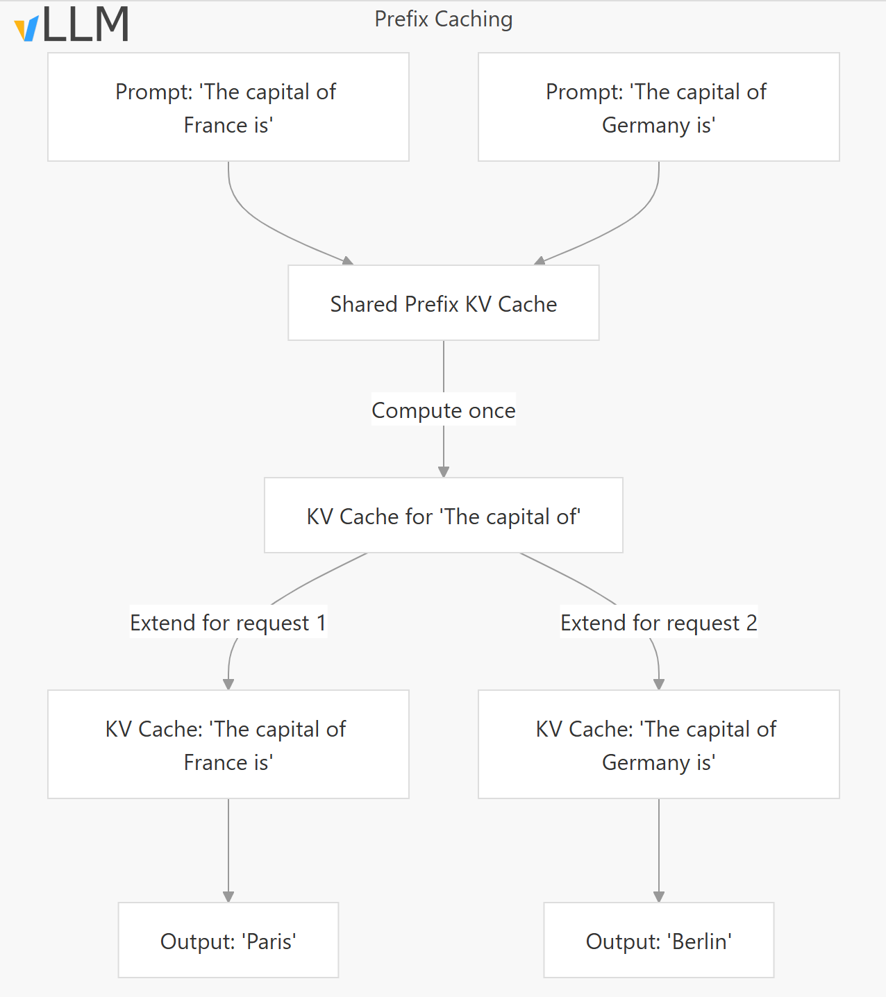
• Cache Reuse: Reuses KV cache for common prefixes across requests
• Computation Saving: Avoids recomputing attention for shared prefix tokens
• Memory Efficiency: Reduces memory usage by sharing KV cache blocks

4. Continuous Batching

In traditional batching, all requests are grouped and processed together—but the batch has to wait for the slowest request to finish. So if one request only needs 1 token and another needs 50, the fast one sits idle, and no new request is accepted, wasting GPU time.  

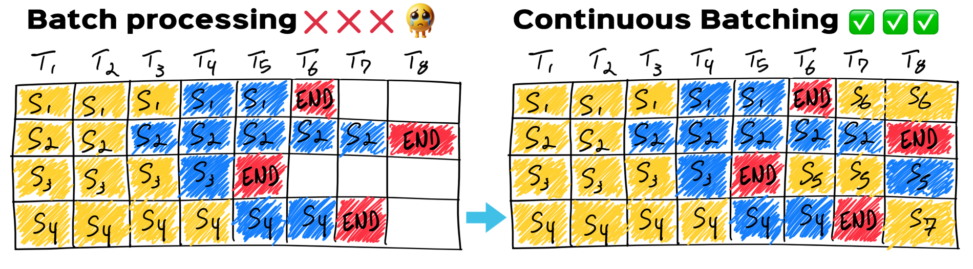
Continuous batching fixes this by

• letting new requests join as others finish in the batch
• keeping the GPU fully used and reducing wait times.
• batches at iteration and not a request level
• Improves latency and throughput

5. Multi-Step Scheduling

Scheduling multiple steps of vLLM’s inner loop allows to dramatically reduce the amount of time spent in scheduling and input preparation (–num-scheduler-steps 8)

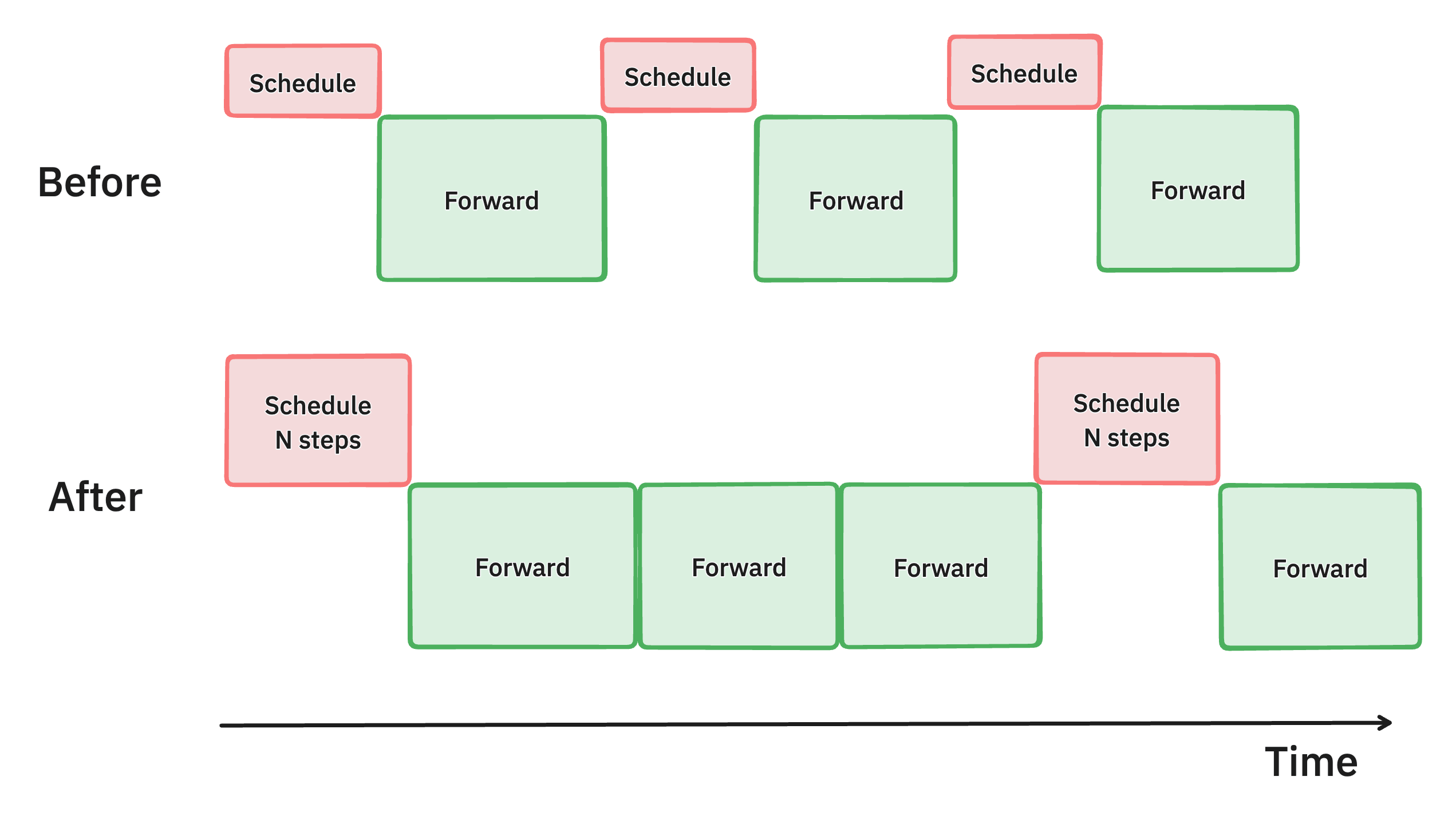
• Reduces bubbles (idle time) on the GPU between each decode step
• Performs scheduling and input preparation once and runs the model for n consecutive steps.
• GPU can continue processing between the n steps without waiting for the CPU

6. Multi-Processing API Server

Initially both API server and LLM Engine were running in the same python process where they would compete for the same CPU cycles, causing contention due to Python’s Global Interpreter Lock (GIL) that prevents true multi-threading. This is fixed with Multi-Processing API Server.

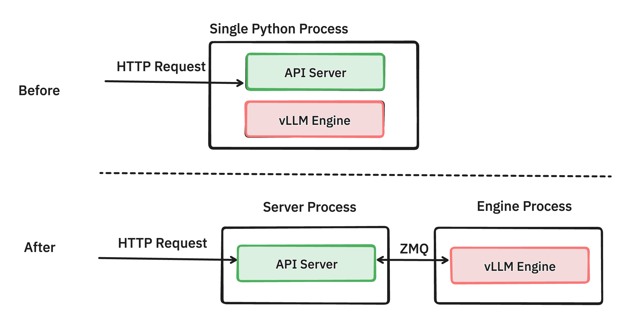
• API/LLM Engine separation allows each component to run in its own Python process, avoiding GIL contention..

III Generation Optimization Layer

1. Speculative Decoding

Speculative decoding is a technique to reduce generation latency by predicting a candidate tokens using a smaller LLM, which are then verified in a batch by a larger mod.

We call the small one Draft runner, and the Big model, target runner with changes in scheduler and memory manager.

⚒️ How it works:

You launch a vLLM server and add parameters to specify the speculative model and the number of tokens to speculate.

1️⃣ A smaller model proposes candidate tokens 🪄
2️⃣ The larger model verifies these tokens in a single batch
3️⃣ This process can generate multiple tokens in a single forward pass, reducing latency

Types of Speculative Decoding

• Draft Model Based: Uses a smaller model to guess tokens ➡️ up to 1.5x speed up
• Prompt Lookup Decoding: Uses the prompt itself to speculate tokens, effective for tasks like summarization.
• 🐍Medusa: Adds extra layers to the original large model to predict multiple tokens.

Performance Considerations

IV.Attention Layer 🧠

Currently, vLLM supports multiple backends for efficient Attention computation across different platforms and GPUs. It automatically selects the most performant backend compatible with your system and model specs. Valid backends are FLASH_ATTN, FLASHINFER or XFORMERS.

1. Flash Attention

Attention is memory-bound, as it spends more time moving data than computing. That’s where FlashAttention solves this by reducing memory access and fusing operations, making attention faster for both training and inference.

It is an IO-aware CUDA implementation that splits attention into smaller tiles processed in fast on-chip memory (SRAM), then writes results back to the high-bandwidth memory (HBM). No HBM back & forth.

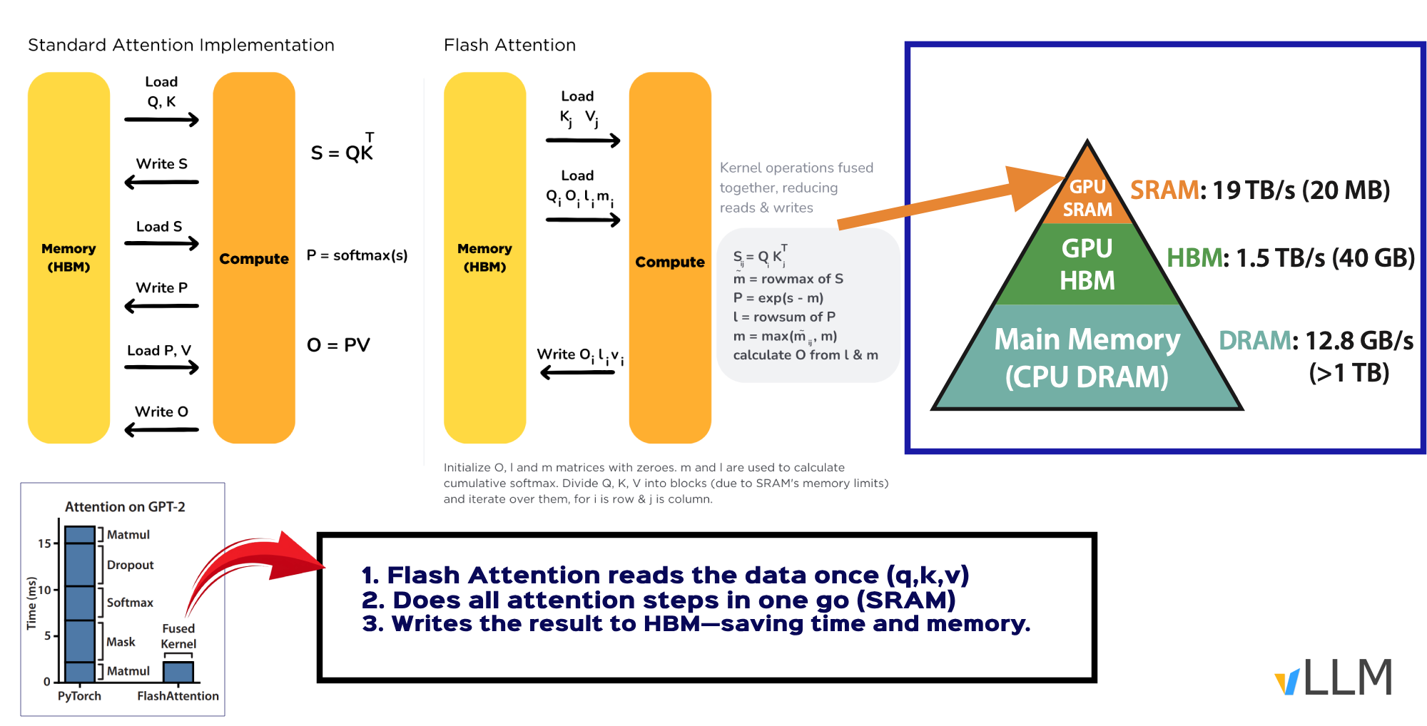
⚒️ How it works:

1️⃣ Flash Attention reads and load the data once (keys, queries, and values) ➡️Tiling
2️⃣ Does all attention steps in one go on-chip (SRAM) ➡️Fusing
3️⃣ Writes the final result back to GPU’s memory (HBM) once.

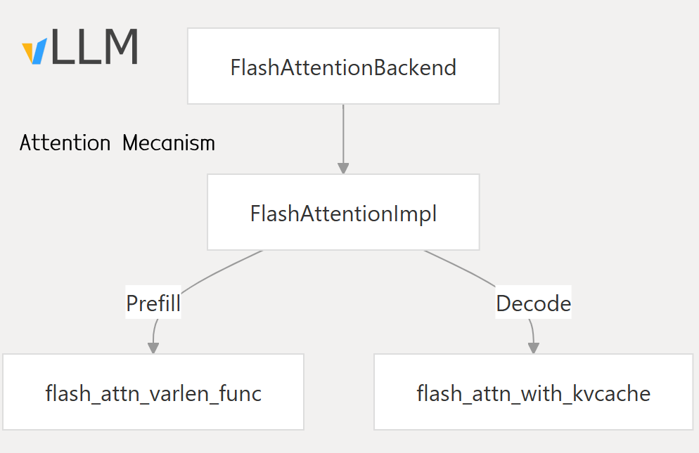
• Works best for long input texts and big batches (prompt/prefill).
• Enabled in vLLM with VLLM_ATTENTION_BACKEND=FLASH_ATTN.
• Automatically chosen by vLLM if your hardware supports it (source).

2. FlashInfer

 FlashInfer, is an implementation designed for faster attention, especially for decoding with paged KV cache and Grouped Query Attention (GQA). It optimizes how the model is served by fusing operations, continuous batching, and prefetching. It tackles KV-cache storage heterogeneity, optimizes memory access and reduce redundancy. 

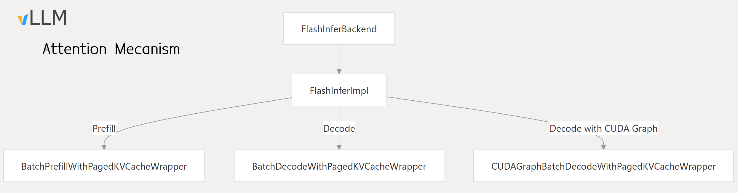
• FlashInfer is a system-level optimization that includes CUDA Graph support for accelerated decoding.
• Uses block-sparse format and to tackle KVCache storage heterogeneity.
• Use advanced scheduling to maximize GPU utilization.
• enabledin vLLM with VLLM_ATTENTION_BACKEND=FLASHINFER.

V. Distributed Inference Layer

Serving large models often leads to memory bottlenecks, such as the dreaded CUDA out of memory error due to:

• ❌ Model cannot fit into a single GPU (i.e llama3_405B ➡️900GB)
• ❌ Model cannot fit into a single node

Distributed Inference solves this by spreading LLM computations across multiple GPUs or nodes for scalability and efficiency.

🎯TL;DR:
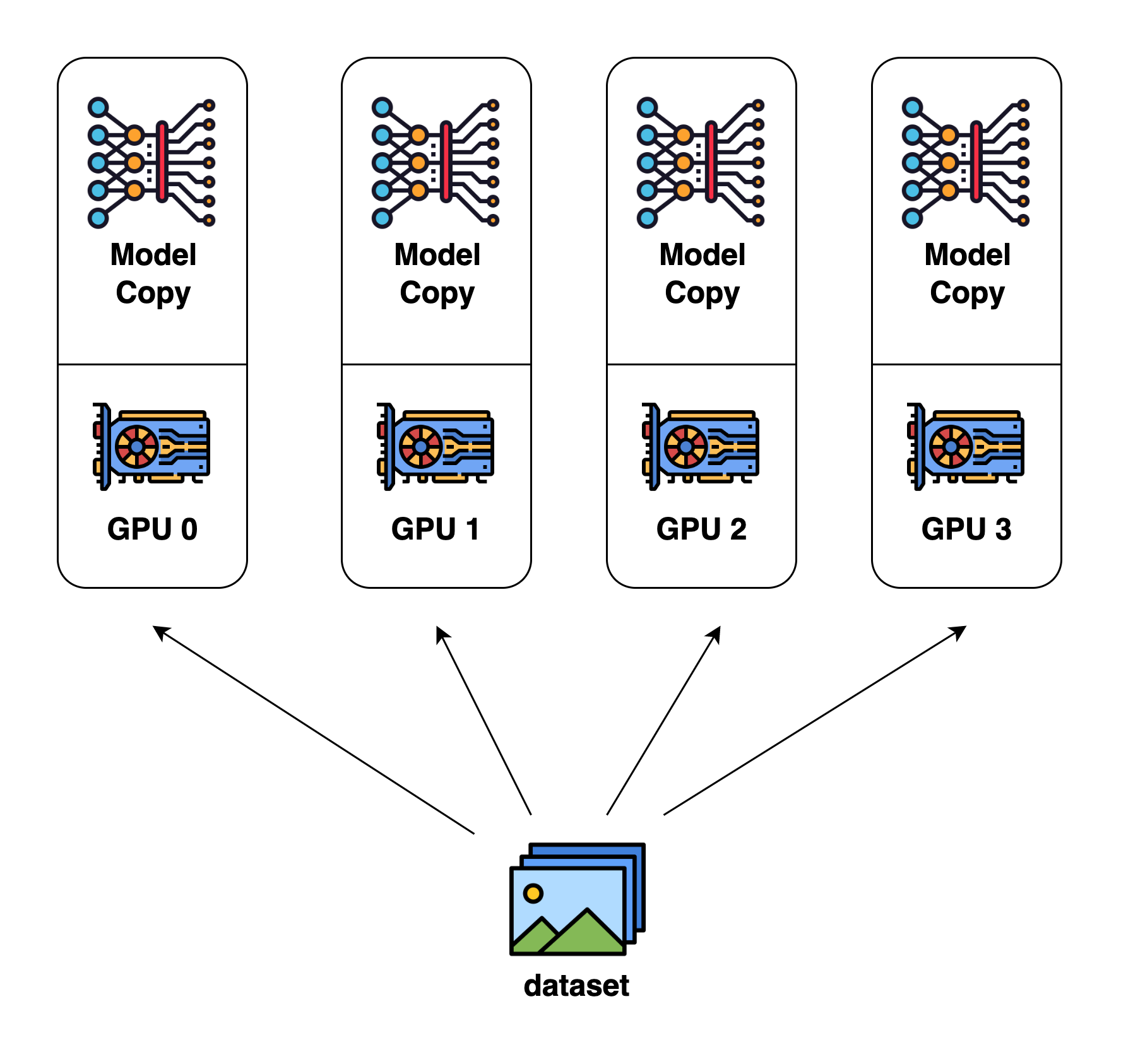
Data parallelism = multiple model copies, Big data to process (training)
Tensor/pipeline = one big model split across GPUs

1. Tensor Parallelism

Tensor parallelism splits a model’s weight matrices across multiple GPUs which enables running big models that wouldn’t fit on a single GPU.

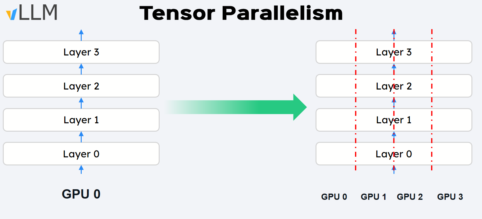
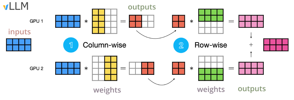
⚒️ How it works

Each GPU gets the same input and computes its share of the layer’s work—like partial matrix multiplications.The results are then combined, allowing a large model to run in parallel when a single GPU isn’t enough.

• Improves end to end latency
• The weight matrices are computed row/column-wise (attention heads & MLP layers shards).
• The vLLM tensor_parallel_size  parameter sets the number of GPUs to use during the parallelism.

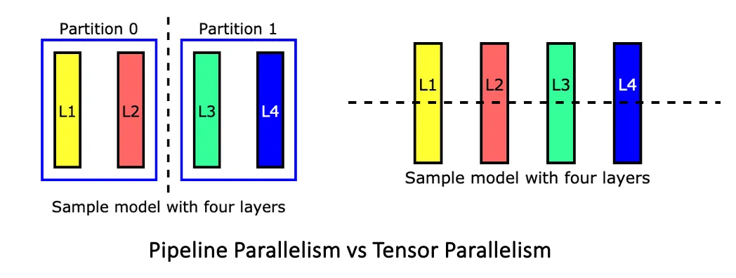
2. Pipeline Parallelism (Multi Node)

 For extremely large models that can’t even fit a single node, tensor parallelism will have high network overhead. Hence Pipeline Parallelism is the answer, as it splits the model vertically (by layers) across different GPUs (each handle one step) .

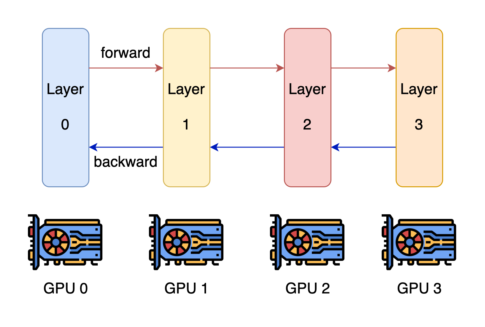
⚒️How it works

• Each GPU has a subset of the layers and only computes for that subset and passes the output to the next GPU.
• An input passe through the first GPU, which processes its assigned layers then passes the intermediate result to next GPU, and so on.
• It has low communication overhead compared to tensor Parallelism.
• Can leverage Chunk-Prefill to keep GPUs active between passes.

Combining Tensor and Pipeline Parallelism 🎯

This hybrid approach maximizes resource utilization and allows for efficient inference and scaling to very large models.

• Within a node➡️ Use tensor parallelism to split computations across GPUs.
• Across nodes➡️ Use pipeline parallelism to assign different layers to different nodes.

$ vllm serve --model deepseek-ai/DeepSeek-R1 \
  --tensor-parallel-size 8 
  --pipeline-parallel-size 2 --max-model-len 16384 \ 
  --enable-chunked-prefill --max-num-batched-tokens 1024 \ 
  --trust-remote-code --gpu-memory-utilization 0.95 --enforce-eager

3. Data Parallelism

When training massive data sets, data parallelism allows to replicate the same model across devices with each GPU processing a subset of the training data, significantly increasing throughput.

🚀Coming Up Next

That wraps up Part 2 of our vLLM for Beginners series, where we explored the key features that make vLLM fast, efficient, and production-ready—from memory optimization techniques to distributed inference.

In the next post, we’ll leave the theory behind and get hands-on—covering everything from CLI-based setup to full-scale deployment using the vLLM Production Stack. Stay tuned for Part 3: Hands-On Deployment with vLLM 🚀

Reference

• vllm_docs
• distributed-inference
• 3D-parallelism

🙋🏻‍♀️If you like this content please subscribe to our blog newsletter ❤️.