Intro
Today, most of us have used nano banana, Midjourney, Kling AI, Luma, or Sora to generate silly videos or catchy images on socials. But what do they share in common? They all rely on Diffusion Models as their core engine, even the brand new Seedance. While many of these are proprietary, the open-source world has exploded with high-quality models that allow anyone, from hobbyists on ComfyUI to enterprises on vLLM-omni, to run their own multimodal platforms.
Following our vllm-omni deep dive, this blog explores how these models actually work in practice.
💡More Logic less mathing
My goal isn’t to bury you in deep math, but to demonstrate the logic behind the basics. I’ll use simplified annotations to ensure that even without a PhD, you’ll walk away understanding the “Big Picture” of AI media generation.
It is my attempt to translate popular publications. You can learn the math side of it in this amzing video By Welsh Labs
I. What is Diffusion in AI?
In physics, diffusion is what happens when you drop ink into water or leave perfume in a room: it spreads, it fills the space, it doesn’t reverse. Structure dissolves into chaos, and entropy wins. Diffusion models expand on this natural phenomenon by learning how to run it backwards. From sharp image to noise (train), and back again (inference).
Hence the two-act story: first you destroy, then learn to create. The magic isn’t in the noise, but teaching a model to find order within it. Precisely what Michelangelo’s metaphor captures: forward diffusion hides the statue inside the marble, reverse diffusion carves it free, one step at a time, guided by your prompt. Can’t have the 2nd without the first.
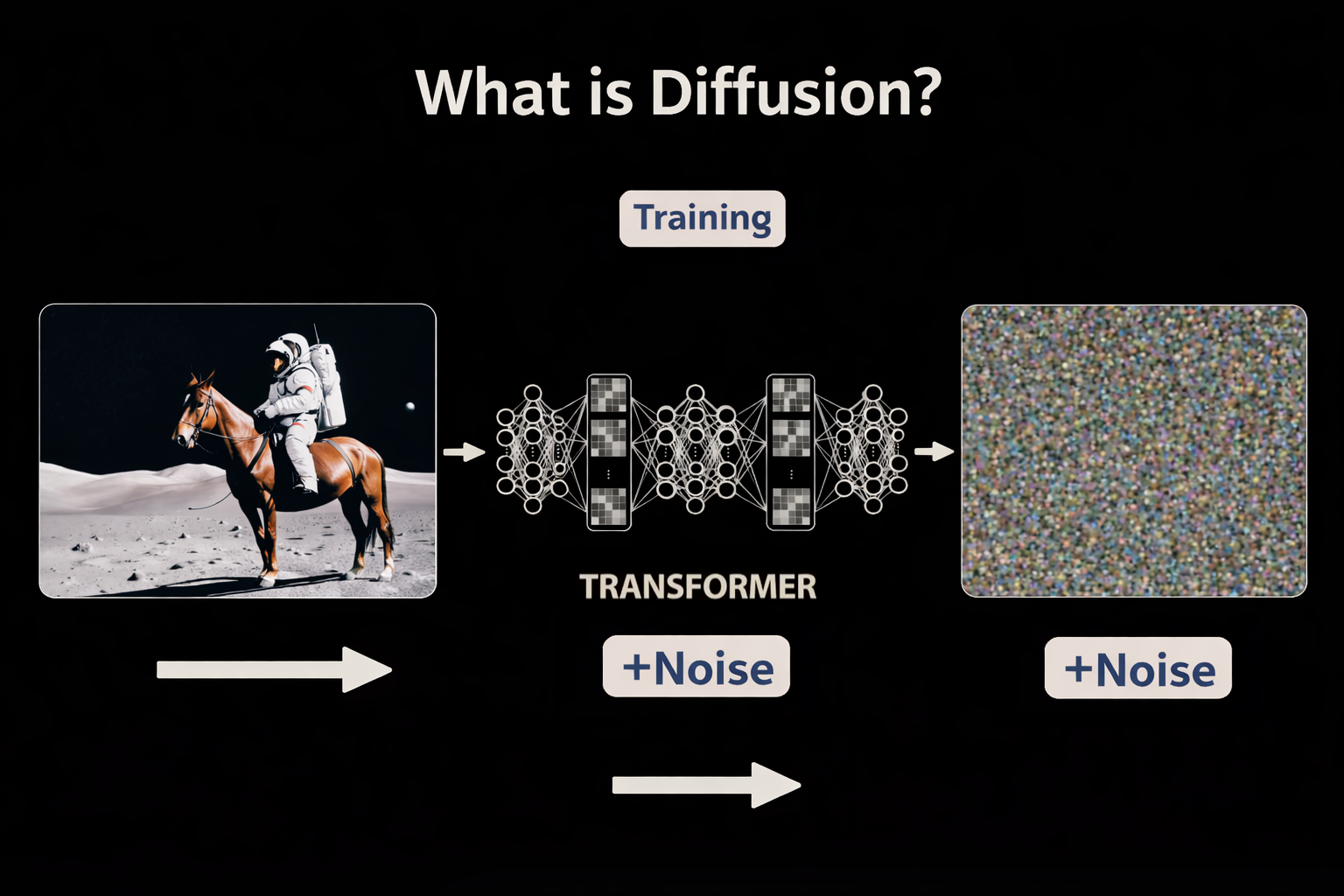
1. Forward Diffusion (Training)
During training, real images are gradually corrupted, by adding tiny amounts of random noise over 100s of steps, until the original image is pure noise. Each step creates a data point: (image, how noisy it is, what noise was added). Text descriptions are encoded and paired with their corresponding images to build the full training corpus.

- Start: A real image or video paired with its text description (i.e “a golden retriever on a beach.”)
- Destroy: Add a tiny amount of noise. Record the result. Repeat multiple of times, until nothing remains but static.
- Finish: Pure noise (random pixels).
- Training loss is typically MSE(Mean Squared Error) between predicted ε(noise) and true ε
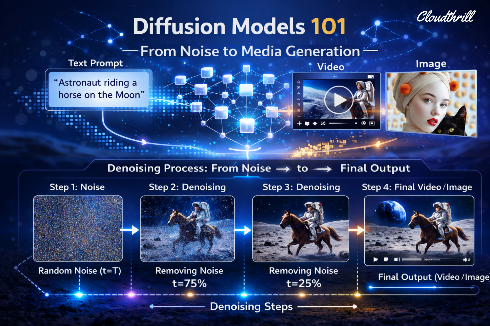
2. Reverse diffusion (inference)
Diffusion generation is like un-blurring a photo step by step. You aren’t “drawing” from scratch; you’re sculpting an image out of a block of marble made of static, guided by your prompt.

- Start: Pure noise (random pixels).
- Denoise(refine): Gradually remove “noise” over many steps guided by text embeddings (your prompt).
- Finish: A clear, high-fidelity image or video.
3. Latent Space(VAE): Diffusion’s ZIP File
Processing a 4K video frame-by-frame is a computational suicide mission. But in 2022, “High-Resolution Image Synthesis with Latent Diffusion Models“ paper — which gave birth to Stable Diffusion — changed the game with VAE (Variational Autoencoder): a high-powered zipper for visual data.
II. Inside a Diffusion Step
Every concept below lives inside one place: the “Denoising Loop” — running hundreds of times per generation, and showing where the GPU cycles are being spent. Before diving into diffusion paths, we must understand the loop first.
1. Timesteps
Timesteps are simply step numbers in the denoising process, a counter that tells the model exactly where it is in the journey from noise to image. The model uses this number to calibrate how aggressively to denoise: early steps make big structural changes, late steps refine fine details.
2. Text Embeddings — The “Brain”
Your prompt (i.e., “A cat in a space suit“) is turned into a vectors called embeddings that encodes meaning and guide the denoising process. So the model doesn’t just make a random pretty picture—it makes yours.
3. Timestep Embeddings — The “GPS”
At every step, a Timestep Embedding (GPS signal) is generated. It helps the model decide what noise to remove, by signaling how noisy the current state is in the noise to image journey. The timestep is encoded into its own embedding alongside the image and text and injected into every transformer block (transformer layer) as a modulation signal.

In the diagram: the Timestep Embedding modulates the Noisy Input through two operations before anything else runs:
Shift (+)— It adjusts the bias of the data (addition).
Scale — It adjusts the “volume” or strength of the features (multiplication).
This re-wires each transformer block at every step — Step 1000 focus on global shapes, Step 10 on fine textures.
"t" (“denoising progress bar”, i.e step 500).
"t_emb" (translated progress bar i.e. step 500, into a “time-aware” vector).
t_emb  = TimestepProjection(t)               ← encode the step number
output = Scale(t_emb) · x + Shift(t_emb) ← modulate the noisy input4. Vector Fields
At each denoising step, the model outputs a vector — a direction and magnitude pointing toward cleaner data. Across the entire latent space, these vectors form a field: a map of which way to move from any noisy state to reach a coherent image. This is the navigation system introduced in Section I.

The text embedding steers which region of that field you’re navigating toward. Timestep tells you how far you’ve come.
5. Unconditional vs. Conditional (prompt)

Without a prompt, the model generates freely — no destination, no instruction, meaning you get a totally random image or video. When a text prompt is added, the model computes a directed prediction, steering toward the concept your words describe. The difference between those two predictions is what makes guidance possible.

-
f(x,t)— is the unconditional prediction, drifting toward “NOT CATS.” f(x,t, cat)— is the conditional prediction, pointing toward the CATS cluster.- The green arrow is the difference between them. No scale applied yet, just two directions, and their gap.
6 Classifier-Free Guidance (CFG)
CFG amplifies that difference. It takes the green arrow and scales it by a guidance weight w — pushing the result harder toward your prompt and further from the generic baseline. Think of it as a creativity vs. control knob: low values give the model freedom, high values enforce the prompt literally.

CFG Formula
\epsilon_{guided} = \underbrace{f(x,t)}_{\text{unconditional prediction}} + \underbrace{w}_{\text{scale}} \cdot \underbrace{\color{green}{[f(x,t,cat) – f(x,t)]}}_{\text{prompt direction}}
\)
7. Negative Prompts

While CFG uses an unconditional prediction as its baseline — steering away from “nothing”. Wan model takes it even further by using Negative prompts and replacing that neutral baseline with something explicit: a description of “what you don’t want“. The model now steers away from a blacklisted concept rather than just away from nothing.
Negative Prompt Formula
\epsilon_{guided} = \color{green}{f(x,t, \text{prompt})} + \underbrace{\alpha}_{\text{scale}} \cdot [\color{green}{f(x,t, \text{prompt})} – \color{red}{f(x,t, \text{neg prompt})}]
\)
III. Diffusion Paths (Solvers)
Every diffusion model starts with pure noise and ends with a coherent image. The question that divided researchers for years: what’s the best path between the two? Three generations of solvers answered that question very differently.
1. DDPM (Denoising Diffusion Probabilistic Models)
📄 Paper Denoising Diffusion Probabilistic Models — Ho et al., 2020 ↗DDPM is like walking home drunk—random steps with few kicks, but you get there with some correction.

How it works:
The original diffusion solver. At every step, the model removes some noise then immediately adds a small random kick back in. Like a stroller stumbling home: moving in the right direction, but shuffling sideways at every step. It eventually reaches the destination, but the path is chaotic and expensive — requiring ~100+ steps minimum. The randomness isn’t a bug — different stumbles = different images from the same prompt. But it also meant you couldn’t skip steps.
DDPM Formula — SDE (Stochastic Differential Equation)
x_{t-1} = x_t + \underbrace{a_t \epsilon_\theta}_{\text{Correction}} + \underbrace{\color{orange}{\eta w_t}}_{\text{Noise}}
\)
DDPM — Full Step Walkthrough
2. DDIM (Deterministic Diffusion Implicit Models)
DDIM is like skiing back home — a predictable slide but faster with smooth curves minus the random kicks.
📄 Paper Denoising Diffusion Implicit Models — Song et al., 2021 ↗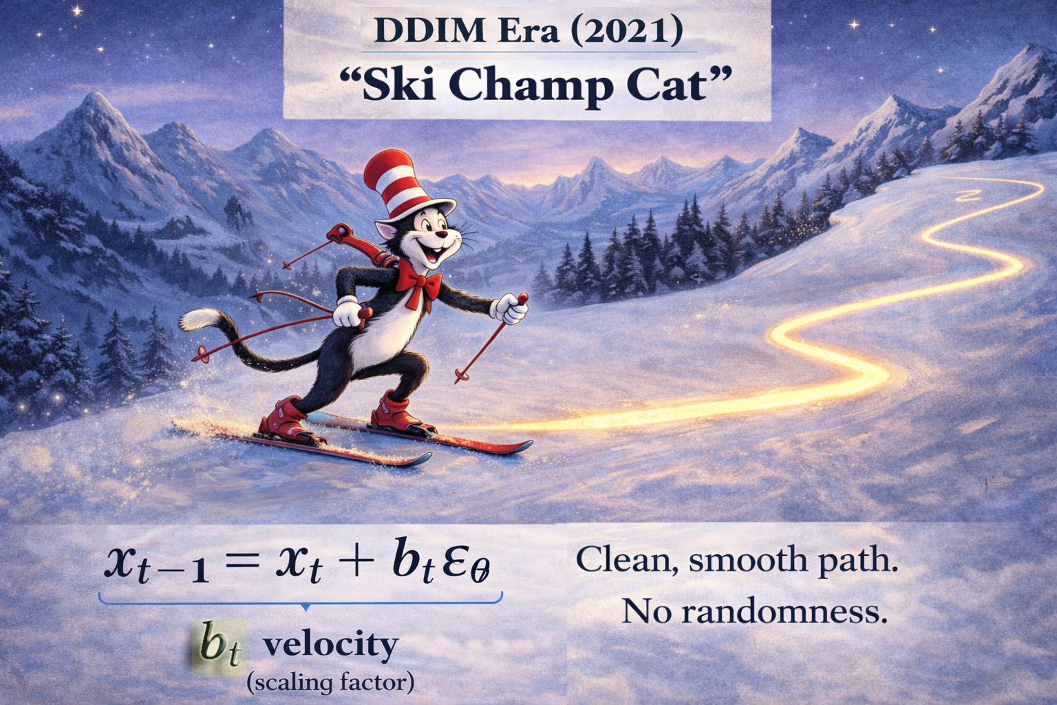
How it works:
Song et al. asked one question: what if we removed the random stumble entirely? DDIM replaced the stochastic process with a deterministic ODE — the model carves a smooth, predictable curve toward the destination. No random kicks. Same starting noise + same prompt = same image every time. And because the path is smooth, you can skip steps (larger leaps)— reducing 100s steps to 50 without losing noticeable quality.
DDIM Formula — ODE (Ordinary Differential Equation)
\underbrace{x_{t-1} = x_t + b_t \epsilon_\theta}_{\text{Reverse Diffusion Step}}
\)
3. Flow Matching
Flow matching is like riding a “Bullet Train” — Straightening the path for maximum speed. Predicting velocity, not noise.
📄 Paper Flow Matching for Generative Modeling — Lipman et al., 2023 ↗
How it works:
DDIM smoothed the path. Flow Matching is when you turn that “Curve” into a “straight Line”. Instead of predicting noise to remove at each step, the model learns to predict a velocity vector — the direct direction from noise to image in a straight line. No randomness, no curves, just the straightest possible path with a consistent speed. Fewer steps, less compute, better quality. This is the solver powering Wan 2.1, Hunyuan, and FLUX today. Perfect for diffusion caching.
Flow Matching Formula (ODE)
x_{t-1} = x_t – \underbrace{\color{green}{\Delta t}}_{\text{StepSize}} \cdot \underbrace{\color{blue}{v(x,t)}}_{\text{Velocity}}
\)
Flow Matching — Full Step Walkthrough
Solvers Comparison Table
IV. The Architecture Evolution 🚀
Every diffusion model needs two things: 1.Something to generate and 2.Something to understand what you asked for. So far we covered the generation side. This section covers the language understanding sid, and how it evolved from basic to genuinely intelligent.
1. CLIP (OpenAI, 2021) — Giving the Model “Eyes”
CLIP encodes image and text into shared embedding space. It has no “hands” to draw; it only has “eyes” to see.
📄 Paper Learning Transferable Visual Models From Natural Language Supervision — Radford et al., 2021 ↗
How it works:
Before CLIP, images and text lived in separate worlds. CLIP changed that by training on 400 million image-text pairs, learning to map both into a shared embedding space. A photo of a cat and the words “a cat” end up together in that space. A photo of a dog ends up far away. This gave diffusion models their first real “eyes”, a way to understand what a prompt means visually. The embedding from CLIP is what gets fed into the denoising loop as the conditioning signal.
2. Imagen (Google, 2022) — Giving the Model a “Brain”
Meet Google’s Imagen … the discovery that replaced the model’s eyes (VLM) with a brain (LLM).
📄 Paper Photorealistic Text-to-Image Diffusion Models with Deep Language Understanding — Saharia et al., 2022 ↗
How it works:
CLIP struggled with complex language (nuanced prompts, spatial relationships, etc). But Google team asked: what if instead, we used an LLM already trained on the complexity of human text? The answer was T5, an LLM trained on text alone and revealed something surprising: a model that had never seen an image still produced far better prompt understanding than CLIP. The “brain” didn’t need to see to understand.
V. The Jump to Video
Images are a single point in time. Video is a sequence of them, and keeping that sequence coherent, consistent, and physically plausible is a completely different problem. These two papers defined how diffusion crossed that threshold.
1. VideoPoet (Google, 2023) — The “LLM for Video”
📄 Paper VideoPoet: A Large Language Model for Zero-Shot Video Generation — Kondratyuk et al., 2023 ↗
multi video generation tasks
How it works:
VideoPoet treated video frames the same way a language model treats words, as tokens in a sequence. By tokenizing video into discrete units and training a transformer to predict the next token, it showed that the same architecture powering text generation could handle temporal coherence in video. No special video-specific architecture needed. Just a big enough transformer and the right tokenization.
2. Lumiere (Google, 2024) — Space-Time Diffusion
Google took Imagen and ditched jitter by adding temporal layers to generate the entire video at once.
📄 Paper Lumiere: A Space-Time Diffusion Model for Video Generation — Bar-Tal et al., 2024 ↗
How it works:
Frame-by-frame video generation’s problem is flicker, the frames are sharp but still unaware of each other. Lumiere solved this with a Space-Time U-Net which generates the entire video frames as a single 3D block (Height × Width × Time), treating time as just another dimension. With features like Consistent stylization and Inpainting.

It uses Temporal Downsampling: reading the “compressed” motion blueprint of the entire clip simultaneously before filling in the details. The model knows where the ball lands at frame 80 before frame 1 is finished.
Conclusion
That’s a wrap — five sections, zero PhD required. If you made it here, congratulations 🏅.
You now understand what most practitioners take ages to piece together: why noise is added before it’s removed, why the path shape matters, why your prompt becomes a vector, and why Google had to inflate an image model just to make video stop flickering.
This was my attempt to translate the papers so you don’t have to read them. The logic was always there — it just needed a drunk stroller and a bullet train to make it click.
Next up: Diffusion caching — TeaCache. Stay Tuned

Run AI Your Way — In Your Cloud
Want full control over your AI backend? The CloudThrill VLLM Private Inference POC is still open — but not forever.
📢 Secure your spot (only a few left), 𝗔𝗽𝗽𝗹𝘆 𝗻𝗼𝘄!
Run AI assistants, RAG, or internal models on an AI backend 𝗽𝗿𝗶𝘃𝗮𝘁𝗲𝗹𝘆 𝗶𝗻 𝘆𝗼𝘂𝗿 𝗰𝗹𝗼𝘂𝗱 –
✅ No external APIs
✅ No vendor lock-in
✅ Total data control
𝗬𝗼𝘂𝗿 𝗶𝗻𝗳𝗿𝗮. 𝗬𝗼𝘂𝗿 𝗺𝗼𝗱𝗲𝗹𝘀. 𝗬𝗼𝘂𝗿 𝗿𝘂𝗹𝗲𝘀…
🙋🏻♀️If you like this content please subscribe to our blog newsletter ❤️.